
|
|
Exploring the Atmosphere With Lidar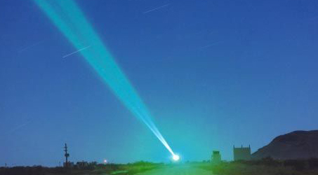 Professor R. Sica What's a Lidar?A lidar is similar to the more familiar radar, and can be thought of as a laser radar. In a radar, radio waves are transmitted into the atmosphere, which scatters some of the power back to the radar's receiver. A lidar also transmits and receives electromagnetic radiation, but at a higher frequency. Lidars operate in the ultraviolet, visible and infrared region of the electromagnetic spectrum.  Different types of physical processes in the atmosphere are related to different types of light scattering. Choosing different types of scattering processes allows atmospheric composition, temperature and wind to be measured. LIDAR is an acronym which stands for LIght Detection And Ranging (radar is also an acronym). A simplified block diagram of a lidar contains a transmitter, receiver and detector system. The lidar's transmitter is a laser, while its receiver is an optical telescope. The basic operation of a laser is described here. Different kinds of lasers are used depending on the power and wavelength required. The lasers may be both cw (continuous wave, on continuous like a light bulb) or pulsed (like a strobe light). Gain mediums for the lasers include, gases (e.g. HeNe = Helium Neon or Xenon Fluoride), solid state diodes, dyes and crystals (e.g. Nd:YAG = Neodymium:Yttrium Aluminum Garnet). For some lidar applications more than 1 kind of laser is used. Here is the transmitter for Western's Purple Crow Lidar, which uses both cw and pulsed lasers. The final output of both channels of the transmitter is pulsed with a pulse repetition rate of 20 times per second and a pulse width of about 7 ns (1 ns = 1 x 10⁻⁹s) . The receiving system records the scattered light received by the receiver at fixed time intervals. Lidars typically use extremely sensitive detectors called photomultiplier tubes to detect the backscattered light.  Photomultiplier tubes (shown below) convert the individual quanta of light, photons, first into electric currents and then into digital photocounts which can be stored and processed on a computer. Amazing when you consider the electric currents generated are on the order of picoamps (1 pA = 10-12 A; a 60 W light bulb draws a current of 0.5 A!). The photocounts received are recorded for fixed time intervals during the return pulse. The times are then converted to heights called range bins since the speed of light is well known. So to find range bins from time: where c is the speed of light, 3 x 10⁸ m/s. So if each range bin is 160 ns long the height of each bin is 24 m. The range-gated photocounts are then stored and analyzed by a computer. Sources for information in this section can be found here. What Important Problems in Atmospheric Science Can Lidar Contribute To?Atmospheric Composition:Air is composed mostly of molecular nitrogen (78%) and molecular oxygen (21%). Other gases in the air are called a minor constituents. Minor constituents are typically measured is parts per million and parts per billion (1 ppm of ozone means 1 ozone molecule for every 1,000,000 air molecules). Don't let the name fool you; some minor constituents are of major importance! Important minor constituents include greenhouse gases such as water vapour, carbon dioxide, methane, chloroflurocarbons (CFCs) and ozone. An ozone molecule is made from 3 oxygen atoms in the following configuration:  Ozone (O3) is important because:
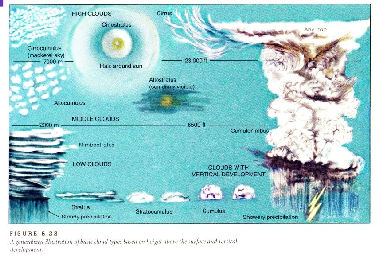
Clouds: Clouds are formed by the ascent of moist air in the lower atmosphere. Different kinds of clouds form a different altitudes and are an indicator of atmospheric stability. The arrival of different types of clouds helps us to predict the next day's weather. Clouds are the least understood piece of the climate change puzzle. Dynamics:
Weather Forecasting:Understanding the above processes (and others) is necessary to develop predictive models for short-term weather (days, months) and long-term weather, which is more properly called climate (decades, centuries). The final "product" of atmospheric science is improving the understanding of physical processes which can then by incorporated in forecast models. Sources for information in this section can be found here. How Can Lidar Measurements Address These Problems?To highlight how lidars can contribute to the scientific problems discussed above we will look at some state-of-the-art lidar systems currently in operation. These four systems are similar in that they all use lasers for transmitters and telescopes of various sizes for their receivers. However, they each use a different type of scattering to address one of the science problems discussed above. DIAL: Measuring ozoneDIAL stands for DIfferential Absorption Lidar. DIAL systems are based on the fact that the absorption of light by the atmosphere is different at different wavelengths.  For ozone the absorption is broad. The laser is tuned between spectral regions of high and low ozone absorption. The difference in absorption of the light at the different wavelengths can be used to determine the amount of ozone. Here is an example of a ozone profile measured by the STROZ-LITE system. Height profiles of ozone are useful form many reasons. For instance, these profiles show the loss of ozone in the Antarctic Ozone Hole. LITE: Detecting Clouds and Aerosols from Space LITE stands for LIdar Technology Experiment. LITE flew on shuttle mission STS-64 in September, 1994. LITE was the first successful demonstration of operating a lidar from space. LITE was designed to measure clouds and aerosols, the small particles of "stuff" in the air that includes cloud droplets. 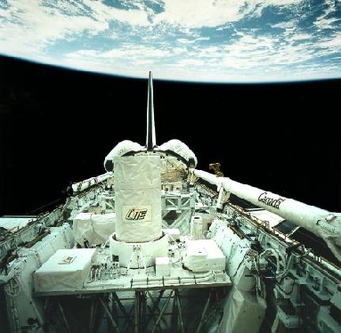 Clouds are measured using elastic scattering of light by the aerosols. Elastic scattering means that the scattered light is at the same frequency as the incident light. Operating a lidar from space allows large regions of the atmosphere to be rapidly sampled. An example of LITE measurements over the Sahara Desert shows the coverage afforded by measurements from space. GALE: An Advanced Wind Lidar GALE stands for Giant Aperture Lidar Experiment . A layer of alkali metal exists in the 80 - 120 km region of Earth's atmosphere due to the constant influx of meteors, like the one shown in this photo. GALE measures wind, temperature and waves using the resonance fluorescence scattering due to the sodium carried into our atmosphere by these visitors from outer space. Resonance fluorescence scattering means that when the sodium atoms are illuminated at a precise wavelength (589 nm, 1 nm = 1 x 10⁻⁹ m) they become excited and radiate light. The lidar's receiver measures a fraction of this light. By adjusting the wavelength of the transmitted light a tiny amount (1 part in 105 of a wavelength!) the shift of the spectral line from its central wavelength can be measured. The shift in the central wavelength is called the Doppler shift (see it!) and a wind is determined from the Doppler effect (hear it!). GALE can make extremely high precision measurements of wind in the region of atmospheric sodium in part due the use of the large aperture Starfire Telescope. Wind measurements by GALE show the dynamic structure of the upper atmosphere due to wave activity. Notice how the wind changes from 40 m/s westward to 80 m/s eastward from 90 to 97 km altitude. PCL: Western's Atmospheric Lidar SystemPCL stands for Purple Crow Lidar The PCL measures temperature, waves and water vapour. Temperature is measured in two ways, one of which is using sodium resonance-fluorescence scattering as in the GALE system. Temperature is also measured using Rayleigh-scattering from air molecules. Rayleigh-scattered light is responsible for the blue sky we observe on a clear day. Blue light is Rayleigh scattered 5 times more strongly than red light; hence in a clear atmosphere with the sun up we see a blue sky. How can the photocounts measured by the lidar be related to temperature? The lidar equation relates the number of received photocounts to the atmospheric density by the lidar equation: Here An explaination of the z2 factor can be found here. Once the density profile is known the temperature can be found by
Combining the above equations gives a relation between the lidar photocounts and the temperature, albeit:
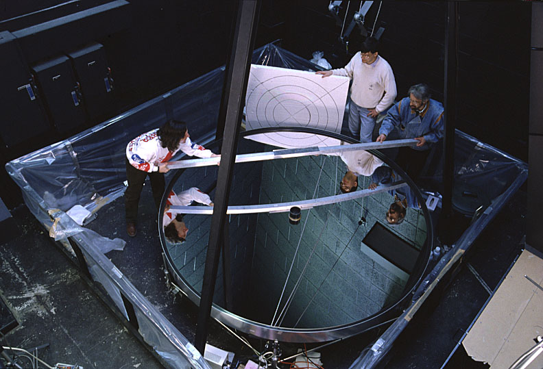
The PCL uses a unique type of receiver called a liquid mirror telescope (LMT). LMTs use a metal that is liquid at room temperature, such as mercury or gallium (mercury for the PCL). The mercury is put in a container and spun, in our case at 6 RPM, to achieve a parabolic surface which is ideal for lidar measurements. A schematic of a LMT system shows the idea is a simple one in principle. Here is our LMT, build with the help of Université Laval and the University of British Columbia. With this technology we can have a mirror larger in diameter (2.65 m) than the Hubble Space Telescope! This large mirror, combined with the laser system shown above, allows our system to measure changes in temperature due to waves in a matter of minutes. Here is an example of a nigthly-averaged temperature profile from the Purple Crow Lidar compared to a model atmosphere. The variations in temperature are due to the action of waves. This figure shows how the temperature can change by tens of degrees in tens of minutes over a night's measurements. I hope you have enjoyed this introduction to lidar. To explore other web sources about lidar start at the Lidar Researchers Directory. References
© 1998, 1999 by Dr. R. J. Sica |