|
|
A Short Primer on Gravity WavesR. J. Sica 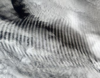 Gravity waves are not something outside your daily experience. Have you ever watched the wake that forms behind a boat? The waves you see are gravity waves. Every noticed the clouds which form in regular bands of cloud and clear sky? These clouds are the result of gravity waves. Gravity waves carry momentum and energy from the troposphere to the middle and upper atmosphere. The gravity waves cause a "drag" on the polar front jet stream, which affects the development of cyclones and anticyclones and thus, the weather on the surface. Gravity waves can also modify the behaviour of the tides in the middle atmosphere and are responsible for the large departure of the middle atmosphere from radiative equilibrium. A special type of gravity wave is a surface wave, which are the waves you see on the surface of a body of water. Often the surface can be quite perturbed with any one spot on the water rising and falling as waves from different directions and sources travel past. The atmosphere is similar, but the waves move vertically as well as horizontally. The idea of gravity waves and their initial theoretical understanding was introduced to an initially skeptical meteorological community by a Canadian scientist, Dr. Colin Hines. His idea of the atmosphere as a soup full of waves has proven correct. A gravity wave is an oscillation caused by the displacement of an air parcel which is restored to its initial position by gravity. The lifting force is buoyancy, while the restoring force is gravity, so a few scientists feel they should be called buoyancy waves! We have discussed gravity, but not buoyancy. Buoyancy is defined by Archimedes' Principle: A body wholly or partially immersed in a fluid will be buoyed up by a force equal to the weight of the fluid that it displaces. The buoyancy force is proportional to the difference in air temperature inside and outside an air parcel. 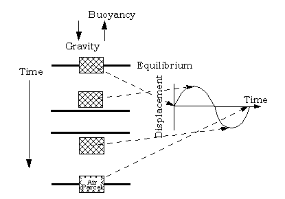
Oscillation of an air parcel, shown on the left, at four "snapshots" in time. The time for the parcel to return to its original position is the buoyancy period. The displacement curve on the right shows the wave motion of the air parcel with time. The time it takes for the air parcel to move back to its starting point after being displaced is called the buoyancy period. The buoyancy period is the shortest period gravity wave that can exist in the atmosphere. Figure 1 shows a picture of an air parcel executing a buoyancy oscillation. Above the troposphere, where the effects of water vapour on the lapse rate are negligible, the buoyancy period, Tb, is given by 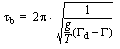 where Γ and Γd are respectively the lapse rate and the dry adiabatic lapse rate. The buoyancy period is smaller in regions of higher atmospheric stability. The buoyancy period increases as the atmosphere becomes more unstable (when the value of Γ approaches the value of Γd in Equation 9.1). Physically, the increase in buoyancy period as an atmosphere becomes more unstable means that, if you displace an air parcel it will oscillate farther from the equilibrium position; thus, it will take longer and longer for the return trip than it would in a stable atmosphere. When the atmosphere is unstable the displaced air parcel will never return and the buoyancy period is infinitely large. In the stratosphere the difference between the lapse rate and the dry adiabatic lapse rate is large and the buoyancy period decreases. The buoyancy period decreases to about 4 min in the stratosphere then increases at the stratopause as the lapse rate changes sign. In the mesosphere the buoyancy period is about 5.5 min, decreasing rapidly in the lower thermosphere as the lapse rate decreases above the mesopause. Energy cascades downward from the 10 km vertical wavelength scale of gravity waves in the mesosphere down to metre scales. The spectrum of gravity waves shows this behaviour (Figure 2). Like the Kolmogorov spectrum of turbulence the curve is a set of straight lines on a log-log plot, so the slope of each line is the exponent of a power law. Figure 2 is drawn for scales appropriate to the mesosphere. At vertical wavelengths greater than about 10 km the gravity wave spectrum depends on the source of the waves. For the source region, the slope of the curve is about -2, though there is little observational evidence at these scales to say this with much certainty. In the source region energy density decreases with wavelength. 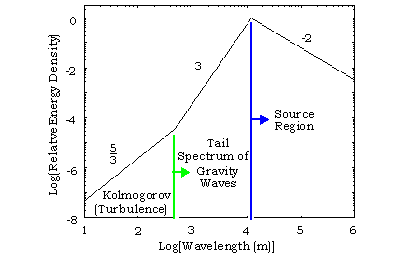
General form of the gravity wave spectrum in the atmosphere. The horizontal axis is the vertical wavelength of the gravity waves, while the vertical axis is the relative energy density (adapted from Gardner et al.). The numbers by the lines indicate the spectral slope in each region. The numbers on the horizontal axis are the power of ten for each tick mark (i.e. 3 means 103 = 1000). The gravity waves of larger scale cascade their energy rapidly to smaller scales until turbulent process continue passing the energy to smaller scales. The next region, between about 100 m and 10 km, is the tail region of the spectrum. According to linear saturation theory, the atmosphere above our heads always appears to contain enough gravity waves dissipating their energy to uniformly fill in the spectrum at all wavelengths, like the spectrum of waves in a small lake full of racing power boats. Numerous measurements show the slope of this region of the spectrum to be about 3. The saturated spectrum is similar in concept to the Kolmogorov spectrum, but in this case the longer wavelength waves carry much more energy than the shorter wavelength waves, since the slope of the saturated spectrum is twice that of the Kolmogorov spectrum. Arguments can be made using linear saturation theory to show that the resulting spectrum of this saturation has a slope of 3. Here is an actual gravity wave spectrum measured in the lower stratosphere by the Purple Crow Lidar, which hints at the complexity of the real world relative to the idealisized explaination given above. 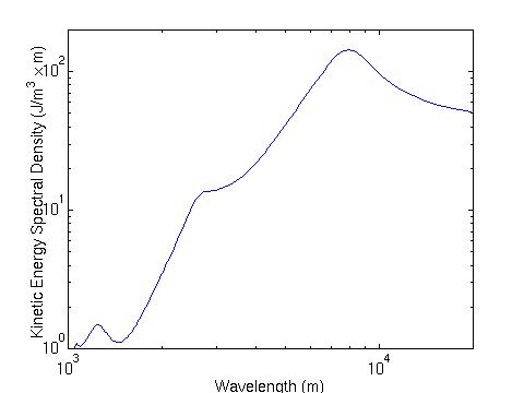 ReferencesAdditional references of interest include the following. Books
Articles
|